Inside an LLM: Weights, Activations, QKV and Training in Motion

What does a language model look like when we arrange its weights in three dimensions? Where is a token ID stored? What changes when the model learns? This lesson follows actual checkpoint values and measured forward passes through three small public models. The controls replay recorded measurements locally; they do not run or train a model in your browser.

Start with three distinct things: weights are persistent numerical parameters; activations are temporary values computed for a particular input; token IDs are integer vocabulary indices assigned by a tokenizer. Training changes the first, which changes how the second is computed from the third.

The visual labs use English controls. Follow the lesson from the whole model, to one head, to one learning step.

1. Three models, three views of computation

Attention, diffusion and MoE describe different aspects of a model. Attention mixes information across token positions. Diffusion describes a corruption-and-reconstruction training and generation process. Mixture of Experts (MoE) routes a token representation through selected feed-forward networks. They can coexist: all three models below use attention, and an MoE can be autoregressive.

Model	Computation in this lesson	Layers	Q / KV heads per layer	Head dimension	Unique parameters
Qwen3-0.6B	Dense, causal	28	16 / 8	128	596,049,920
MDLM-OWT	Masked diffusion, bidirectional	12	12 / 12	64	169,627,218
Granite 3.1 1B-A400M	Causal MoE, 8 of 32 experts per layer	24	16 / 8	64	1,334,625,280

The model names are approximate size labels. Granite stores about 1.33 billion parameters even though only part of its expert capacity is used per token. Qwen’s checkpoint stores its tied input embedding and output head twice: 751,632,384 stored coefficients correspond to 596,049,920 unique parameters. MDLM also stores a 32-scalar positional buffer. Those distinctions matter when counting the contents of a weight file.

2. Rotate the entire model, then replay the input

Select Granite, choose MoE routing weight, and press Play token samples. Each frame selects another recorded token position. Switch to Stored weight RMS: the stored weights remain the same as the selected input token changes. Switch back to activations to see input-dependent values. Drag to rotate, or choose any layer and unit through the menus.

The sentence is shared across models:

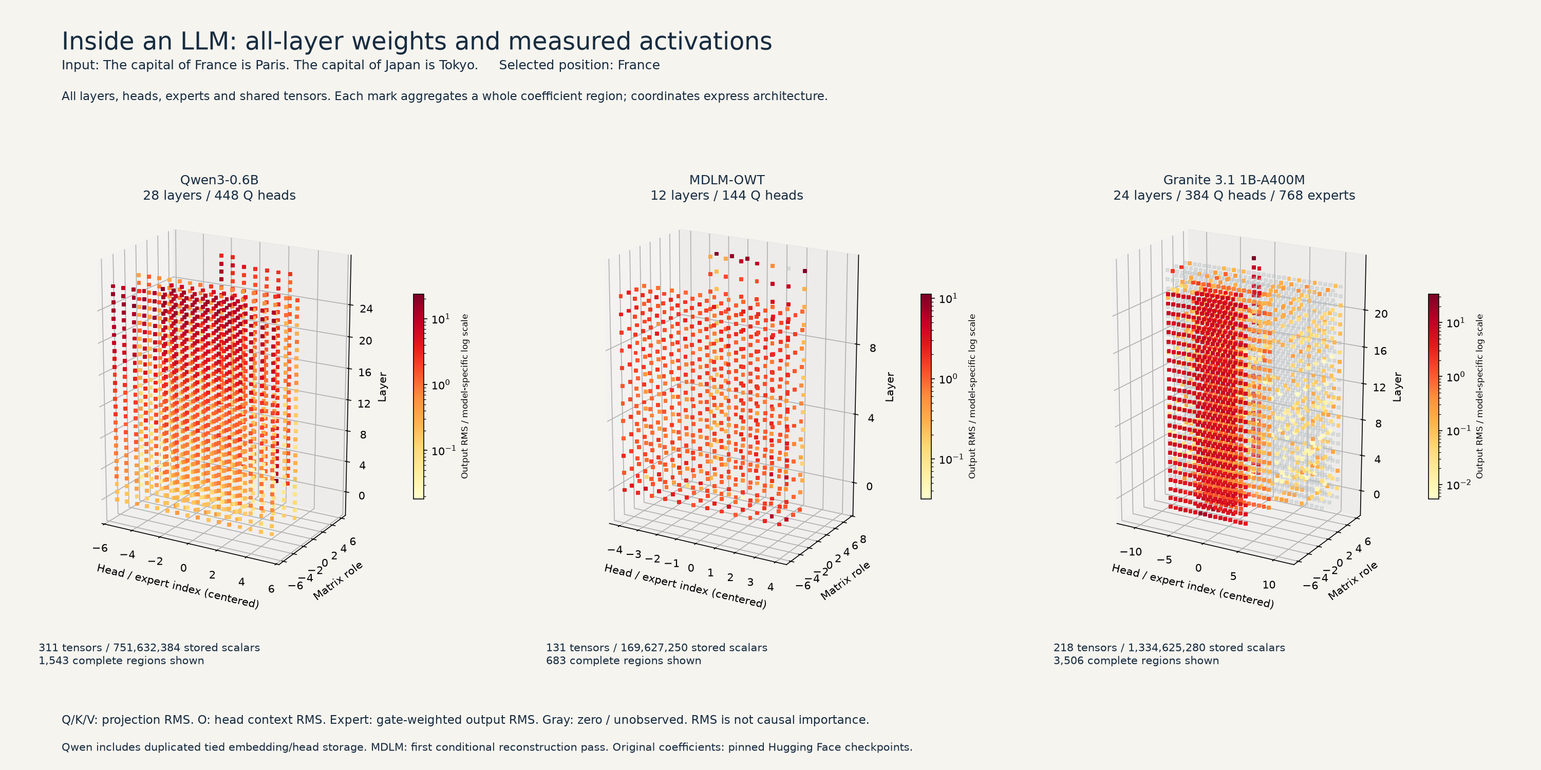
The capital of France is Paris. The capital of Japan is Tokyo.

The atlas covers all 660 stored tensors, partitioned into 5,732 units across every layer, head and expert. Every coefficient belongs to a unit; the view is not a 64 × 64 crop. Each solid aggregates a whole head, expert matrix or shared tensor. It does not render all 2.26 billion stored scalars as separate points. The JSON link inside the lab exposes each region’s original tensor shape, partition, count and statistics; the pinned Hugging Face checkpoints contain the original coefficients.

The coordinates express architecture: layer, head/expert index and matrix role. They are not a learned semantic space. Color has several meanings: Q/K/V projection RMS, head-context RMS for O, or RMS of an expert’s gate-weighted output. Routing mode instead shows actual gate weights. RMS measures magnitude, not causal importance, knowledge content or model quality. The color scale is fixed within each model and differs across models.

Qwen and Granite were run on the complete sentence as causal prefill. Their final next-token predictions were both The; this was not a long generation run. MDLM instead received masks at Paris and Tokyo, then restored Tokyo and Paris in two greedy passes. That is a conditional reconstruction exercise, not a reproduction of its paper’s full diffusion sampler. Token playback scans positions within a recorded forward pass; it is not a movie of tokens moving sequentially through the hardware.

3. Where do token IDs and weights live?

A tokenizer stores the mapping between text pieces and IDs. A piece may be a word, subword, punctuation or byte-related sequence; it need not be one character. The embedding matrix stores a learned vector for each vocabulary index. For the Qwen tokenizer used here, word is ID 3409. That integer selects row 3409 of the embedding matrix. It is an address, not the vector’s numerical content.

text → tokenizer → integer IDs → E[ID] → hidden vectors through layers
     → vocabulary logits → probabilities → selected ID → tokenizer → text

Qwen checkpoint examples:
model.embed_tokens.weight               # vocabulary × hidden dimension
model.layers.0.self_attn.q_proj.weight   # output dimension × input dimension
model.layers.0.self_attn.k_proj.weight
model.layers.0.self_attn.v_proj.weight
lm_head.weight                          # vocabulary × hidden dimension

Intermediate layers transform vectors; they do not each contain another token-ID dictionary. The output matrix has a row corresponding to each vocabulary ID and produces its logit. Qwen and Granite share input/output weights; MDLM uses separate matrices. A checkpoint such as safetensors stores named numerical tensors with shapes, dtypes and byte ranges. It does not contain a permanent table of every input’s activation pattern.

During inference, hidden states and attention values are computed in memory. An autoregressive runtime may retain projected keys and values in a KV cache to avoid recomputing past tokens. That cache is temporary inference state, distinct from learned checkpoint weights.

4. From one input vector to Query, Key and Value

At each attention layer, three learned projections produce Q, K and V. Think of Q as a matching request, K as information used to match, and V as content to combine. These are functional roles, not human-readable labels attached to individual coordinates. The following notation uses the checkpoint convention of output-by-input matrices:

Q = x WQᵀ        K = x WKᵀ        V = x WVᵀ
score(i,j) = scale × dot(Q_attention[i], K_attention[j])
A[i,:] = softmax(masked scores[i,:])
context[i] = Σ_j A[i,j] × V[j]

Here, x is the actual normalized or modulated input to the projections, rather than necessarily the untouched embedding row. Qwen additionally normalizes Q/K by head. All three models rotate Q/K with RoPE to incorporate position; V is not rotated. The stage control separates raw projections from actual attention inputs. Granite’s configured score scale is 0.015625; substituting the usual inverse square root would give different values.

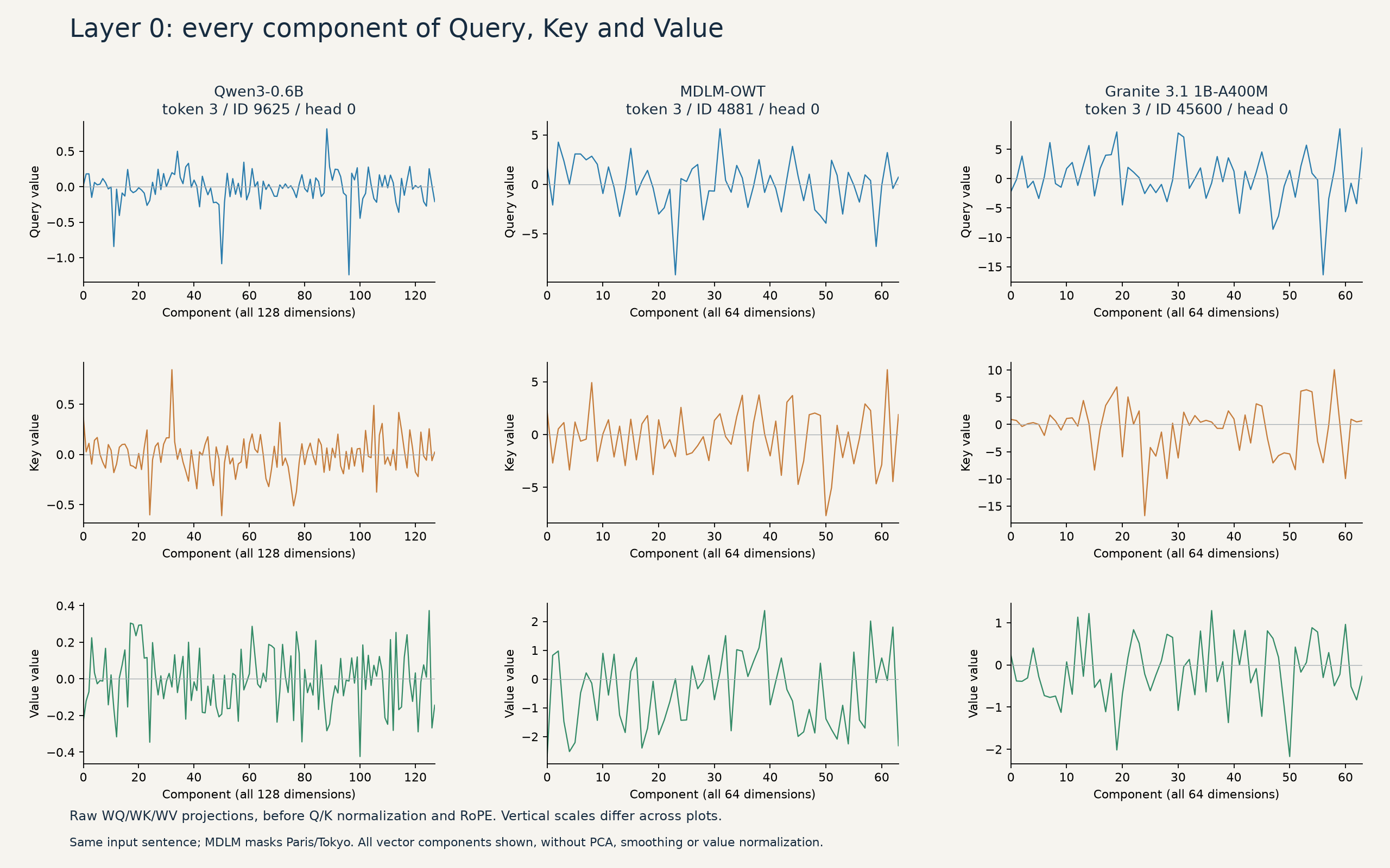
Select Qwen, head 0 and the France token. Move the component slider, expand the full embedding, then switch Query head from 0 to 1. Q changes, while the corresponding K/V head stays shared: 16 Query heads use 8 Key/Value heads in Qwen and Granite. Finally choose a future Key position relative to the Query: causal attention assigns it zero probability. MDLM’s bidirectional attention can use both directions.

This lab displays layer 0, every token and every head, with all 128 or 64 components of each selected vector. It is not PCA and does not discard dimensions. Each chart uses its own vertical scale. Attention bars are always the actual model’s weights after Q/K transformations and masking, even when the upper plots show raw projections.

5. How does training remember a pattern?

The model does not normally save “these characters activated these exact neurons” as a separate record. It computes a loss, differentiates that loss through the operations, and adjusts coefficients. The resulting weights change which future inputs produce which hidden states and predictions. Knowledge and behavior are distributed across many parameters; an activation by itself does not prove where a fact is stored.

For a dense autoregressive model, training usually predicts the next token under a causal mask. For masked diffusion, a training example is corrupted at a sampled noise/masking level and the model learns reconstruction with the objective’s appropriate weighting. For an MoE language model, the language-model loss propagates through selected experts and routing weights; routing regularizers may also contribute. Unselected experts do not receive that token’s ordinary selected-expert contribution. Across many tokens, other experts are selected and trained too.

The next animation follows an actual, deliberately narrow experiment: one example, one SGD update at learning rate 0.01, with dropout disabled. Qwen/Granite predict apple after The secret word is; MDLM reconstructs a masked apple position. We froze the base model and updated one input embedding-row delta and the final layer’s FFN output matrix; Granite also updated its final router. Gradients still travel through frozen layers to reach the trainable embedding delta. This is a partial learning demonstration, not the models’ original pretraining.

Press Play, or use Next to inspect each stage: text → IDs → embedding lookup → all-layer forward → vocabulary scores → loss/backpropagation → update → another forward with the same IDs. The seven stages combine prediction scoring into one scene. Compare Before with Current in the coefficient table. The moving marker and matrix geometry are schematic, while endpoint coefficients, losses and probabilities are measured. Intermediate interpolation is not an observed optimizer trajectory.

Model	Target ID	Cross-entropy before	Cross-entropy after
Qwen3-0.6B	23268	12.416276	0.001918
MDLM-OWT	17180	16.440016	14.581282
Granite 3.1 1B-A400M	38955	8.933086	0.000000119

These numbers show fitting to one training example, not improved general capability. MDLM’s target probability increased from about 7.25e-8 to 4.65e-7 and did not become the most likely prediction. Qwen/Granite’s large probability changes are not evidence of generalization or retention. The same row delta was applied to the input and output paths where embeddings are tied. Original checkpoint files were left unchanged; experimental updates were saved separately. During normal full pretraining, many more parameters receive updates over many batches.

6. What is real, what is drawn, and how to check it

All three complete checkpoints were downloaded at the immutable revisions linked above and verified against their published LFS SHA-256 digests. Every stored coefficient was scanned. The atlas uses whole-region statistics; the QKV lab retains every displayed component losslessly, including BF16 bit patterns. No model weights need to be downloaded by readers.

Qwen and Granite used Transformers 5.4.0, PyTorch 2.6.0, MPS and eager attention with BF16 checkpoint weights for inference. MDLM used its authors’ checkpoint/code with CUDA-specific attention, RoPE and fused operations replaced by equivalent eager Torch equations in F32 on MPS; bitwise equivalence to CUDA kernels was not tested. The partial Granite training run used an exact BF16-to-FP32 conversion because its BF16 backward path was unsupported on MPS. Its objective also included the configured router auxiliary loss; the table reports only cross-entropy.

For these runs, observers changed final logits by zero. Recomputing the first-layer Q/K/V from captured projection inputs and original matrices gave maximum difference zero. Across all layers, recomputed QK scores and Attention × V contexts also matched the recorded values with maximum difference zero. Those checks establish consistency for these implementations and inputs; they do not establish semantic explanations for individual neurons.

The three layouts show the architecture we indexed. They do not establish that dense models, diffusion models and MoEs have three intrinsic geometric shapes. A continuous-diffusion model referred to as Sigma in the original discussion was not analyzed because its canonical public checkpoint was not identified; MDLM is not a substitute measurement of Sigma.

Data and primary sources

• Download manifest and SHA-256 checksums, all-weight coverage verification, QKV numeric verification, and partial-training verification.
• Actual training records: Qwen, MDLM, Granite. Inference environment.
• Original model cards: Qwen3-0.6B, MDLM-OWT, IBM Granite. These models are released under Apache 2.0; the linked repositories provide their terms and attribution.
• MDLM paper and implementation, Attention Is All You Need, safetensors format.

Measurements and lesson prepared November 5, 2026. Interactive labs use modern browsers with DecompressionStream support; the cover and full-component QKV figure provide static views.